OTHER FORMATS
As well as peak property values vs distance, we can find out how a property is distributed in the blast wave at a particular time, when the shock is 100 m from the explosion centre, for example. To find out when the shock is at that position, we can select Shock Arrival Times on the Data Type submenu and display the following:

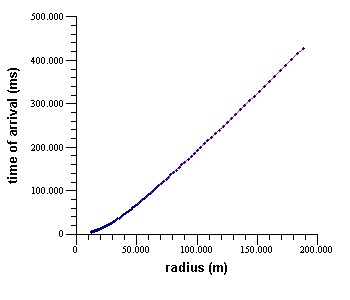
Times of shock arrival, for a 2000 kg ANFO surface burst.

If we use 'Interpolate at X for Y' to obtain the time at which the shock is at 100 metres, we get 192 milliseconds (as on previous page). Let's select Wave Profiles on the Data Format submenu and enter 192 in the dialogue box which appears. We get the following (assuming static overpressures is selected):

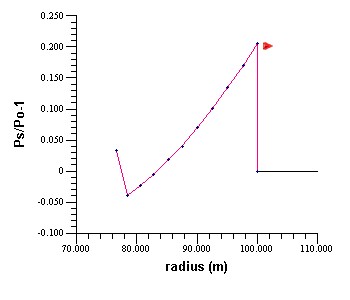
Wave profile of static overpressure at time 192 ms. The shock is at 100 m, travelling to the right (arrow added for illustration). The 'structure' to its left at 77-78 m is a second shock.

Next, we'll display the time history of static overpressure at 100 m, by selecting Time Histories on the Data Format submenu, entering 100 and clicking OK:

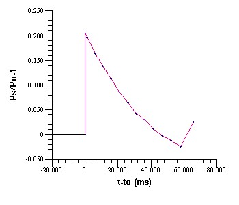
Time history of static overpressure at 100 m. The shock arrives at 192 ms with peak overpressure 0.2056 atm. The second shock arrives about 60 ms later. The Interpolate for Y at X option (Y=0) can be used to obtain the time of positive overpressure duration, 45.93 ms, and the Integrate option used to obtain static overpressure impulse, 3.95 atm-ms. Time histories like the one shown here are measured using electronic pressure transducers.

All of the graphical illustrations on this page can also be displayed numerically. Both graphical and numerical displays can be printed or saved to disk.

Next | Back | Quit